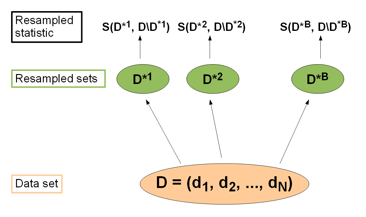
Resampling strategies are usually used to assess the performance of a learning algorithm: The entire data set is (repeatedly) split into training sets \(D^{*b}\) and test sets \(D \setminus D^{*b}\), \(b = 1,\ldots,B\). The learner is trained on each training set, predictions are made on the corresponding test set (sometimes on the training set as well) and the performance measure \(S(D^{*b}, D \setminus D^{*b})\) is calculated. Then the \(B\) individual performance values are aggregated, most often by calculating the mean. There exist various different resampling strategies, for example cross-validation and bootstrap, to mention just two popular approaches.
Resampling Figure
If you want to read up on further details, the paper Resampling Strategies for Model Assessment and Selection by Simon is probably not a bad choice. Bernd has also published a paper Resampling methods for meta-model validation with recommendations for evolutionary computation which contains detailed descriptions and lots of statistical background information on resampling methods.
Defining the resampling strategy
In mlr the resampling strategy can be defined via function makeResampleDesc(). It requires a string that specifies the resampling method and, depending on the selected strategy, further information like the number of iterations. The supported resampling strategies are:
- Cross-validation (
"CV"), - Leave-one-out cross-validation (
"LOO"), - Repeated cross-validation (
"RepCV"), - Out-of-bag bootstrap and other variants like b632 (
"Bootstrap"), - Subsampling, also called Monte-Carlo cross-validation (
"Subsample"), - Holdout (training/test) (
"Holdout").
For example if you want to use 3-fold cross-validation type:
# 3-fold cross-validation
rdesc = makeResampleDesc("CV", iters = 3)
rdesc
## Resample description: cross-validation with 3 iterations.
## Predict: test
## Stratification: FALSE
For holdout estimation use:
# Holdout estimation
rdesc = makeResampleDesc("Holdout")
rdesc
## Resample description: holdout with 0.67 split rate.
## Predict: test
## Stratification: FALSE
In order to save you some typing mlr contains some pre-defined resample descriptions for very common strategies like holdout (hout (makeResampleDesc())) as well as cross-validation with different numbers of folds (e.g., cv5 (makeResampleDesc()) or cv10 (makeResampleDesc())).
hout
## Resample description: holdout with 0.67 split rate.
## Predict: test
## Stratification: FALSE

cv3
## Resample description: cross-validation with 3 iterations.
## Predict: test
## Stratification: FALSE
Performing the resampling
Function resample() evaluates a Learner (makeLearner()) on a given machine learning Task() using the selected resampling strategy (makeResampleDesc()).
As a first example, the performance of linear regression (stats::lm()) on the BostonHousing (mlbench::BostonHousing()) data set is calculated using 3-fold cross-validation.
Generally, for \(K\)-fold cross-validation the data set \(D\) is partitioned into \(K\) subsets of (approximately) equal size. In the \(b\)-th of the \(K\) iterations, the \(b\)-th subset is used for testing, while the union of the remaining parts forms the training set.
As usual, you can either pass a Learner (makeLearner()) object to resample() or, as done here, provide the class name "regr.lm" of the learner. Since no performance measure is specified the default for regression learners (mean squared error, mse) is calculated.
## Resampling: cross-validation
## Measures:             mse
## [Resample] iter 1:    19.8630628
## [Resample] iter 2:    29.4831894
## [Resample] iter 3:    21.2694775
##
## Aggregated Result: mse.test.mean=23.5385766
##
# Specify the resampling strategy (3-fold cross-validation)
rdesc = makeResampleDesc("CV", iters = 3)

# Calculate the performance
r = resample("regr.lm", bh.task, rdesc)
## Resampling: cross-validation
## Measures:             mse
## [Resample] iter 1:    25.1371739
## [Resample] iter 2:    23.1279497
## [Resample] iter 3:    21.9152672
##
## Aggregated Result: mse.test.mean=23.3934636
##

r
## Resample Result
## Task: BostonHousing-example
## Learner: regr.lm
## Aggr perf: mse.test.mean=23.3934636
## Runtime: 0.0375051
The result r is an object of class resample() result. It contains performance results for the learner and some additional information like the runtime, predicted values, and optionally the models fitted in single resampling iterations.
# Peak into r
names(r)
##  [1] "learner.id"     "task.id"        "task.desc"      "measures.train"
##  [5] "measures.test"  "aggr"           "pred"           "models"
##  [9] "err.msgs"       "err.dumps"      "extract"        "runtime"

r$aggr
## mse.test.mean
##      23.53858

r$measures.test
##   iter      mse
## 1    1 19.86306
## 2    2 29.48319
## 3    3 21.26948
r$measures.test gives the performance on each of the 3 test data sets. r$aggr shows the aggregated performance value. Its name "mse.test.mean" indicates the performance measure, mse, and the method, test.mean (aggregations()), used to aggregate the 3 individual performances. test.mean (aggregations()) is the default aggregation scheme for most performance measures and, as the name implies, takes the mean over the performances on the test data sets.
Resampling in mlr works the same way for all types of learning problems and learners. Below is a classification example where a classification tree (rpart) (rpart::rpart()) is evaluated on the Sonar (mlbench::sonar()) data set by subsampling with 5 iterations.
In each subsampling iteration the data set \(D\) is randomly partitioned into a training and a test set according to a given percentage, e.g., 2/3 training and 1/3 test set. If there is just one iteration, the strategy is commonly called holdout or test sample estimation.
You can calculate several measures at once by passing a list of Measures (makeMeasure())s to resample(). Below, the error rate (mmce), false positive and false negative rates (fpr, fnr), and the time it takes to train the learner (timetrain) are estimated by subsampling with 5 iterations.
# Subsampling with 5 iterations and default split ratio 2/3
rdesc = makeResampleDesc("Subsample", iters = 5)

# Subsampling with 5 iterations and 4/5 training data
rdesc = makeResampleDesc("Subsample", iters = 5, split = 4/5)

# Classification tree with information splitting criterion
lrn = makeLearner("classif.rpart", parms = list(split = "information"))

# Calculate the performance measures
r = resample(lrn, sonar.task, rdesc, measures = list(mmce, fpr, fnr, timetrain))
## Resampling: subsampling
## Measures:             mmce        fpr         fnr         timetrain
## [Resample] iter 1:    0.4047619   0.5416667   0.2222222   0.0110000
## [Resample] iter 2:    0.1666667   0.1200000   0.2352941   0.0070000
## [Resample] iter 3:    0.3333333   0.1333333   0.4444444   0.0100000
## [Resample] iter 4:    0.2380952   0.3913043   0.0526316   0.0280000
## [Resample] iter 5:    0.3095238   0.2800000   0.3529412   0.0080000
##
## Aggregated Result: mmce.test.mean=0.2904762,fpr.test.mean=0.2932609,fnr.test.mean=0.2615067,timetrain.test.mean=0.0128000
##

r
## Resample Result
## Task: Sonar-example
## Learner: classif.rpart
## Aggr perf: mmce.test.mean=0.2904762,fpr.test.mean=0.2932609,fnr.test.mean=0.2615067,timetrain.test.mean=0.0128000
## Runtime: 0.10692
If you want to add further measures afterwards, use addRRMeasure().
# Add balanced error rate (ber) and time used to predict
addRRMeasure(r, list(ber, timepredict))

## Resample Result
## Task: Sonar-example
## Learner: classif.rpart
## Aggr perf: mmce.test.mean=0.2904762,fpr.test.mean=0.2932609,fnr.test.mean=0.2615067,timetrain.test.mean=0.0128000,ber.test.mean=0.2773838,timepredict.test.mean=0.0032000
## Runtime: 0.10692
By default, resample() prints progress messages and intermediate results. You can turn this off by setting show.info = FALSE, as done in the code chunk below. (If you are interested in suppressing these messages permanently have a look at the tutorial page about configuring mlr.)
In the above example, the Learner (makeLearner()) was explicitly constructed. For convenience you can also specify the learner as a string and pass any learner parameters via the ... argument of resample().
r = resample("classif.rpart", parms = list(split = "information"), sonar.task, rdesc,
  measures = list(mmce, fpr, fnr, timetrain), show.info = FALSE)

r

## Resample Result
## Task: Sonar-example
## Learner: classif.rpart
## Aggr perf: mmce.test.mean=0.2428571,fpr.test.mean=0.2968173,fnr.test.mean=0.1970195,timetrain.test.mean=0.0084000
## Runtime: 0.0791025
Accessing resample results
Apart from the learner performance you can extract further information from the resample results, for example predicted values or the models fitted in individual resample iterations.
Predictions
Per default, the resample() result contains the predictions made during the resampling. If you do not want to keep them, e.g., in order to conserve memory, set keep.pred = FALSE when calling resample().
The predictions are stored in slot $pred of the resampling result, which can also be accessed by function getRRPredictions().
r$pred
## Resampled Prediction for:
## Resample description: subsampling with 5 iterations and 0.80 split rate.
## Predict: test
## Stratification: FALSE
## predict.type: response
## threshold:
## time (mean): 0.00
##    id truth response iter  set
## 1  18     R        M    1 test
## 2 189     M        M    1 test
## 3  88     R        R    1 test
## 4 121     M        R    1 test
## 5 165     M        R    1 test
## 6 111     M        M    1 test
## ... (#rows: 210, #cols: 5)

pred = getRRPredictions(r)
pred
## Resampled Prediction for:
## Resample description: subsampling with 5 iterations and 0.80 split rate.
## Predict: test
## Stratification: FALSE
## predict.type: response
## threshold:
## time (mean): 0.00
##    id truth response iter  set
## 1  18     R        M    1 test
## 2 189     M        M    1 test
## 3  88     R        R    1 test
## 4 121     M        R    1 test
## 5 165     M        R    1 test
## 6 111     M        M    1 test
## ... (#rows: 210, #cols: 5)
pred is an object of class resample() Prediction. Just as a Prediction() object (see the tutorial page on making predictions it has an element $data which is a data.frame that contains the predictions and in the case of a supervised learning problem the true values of the target variable(s). You can use as.data.frame (Prediction() to directly access the $data slot. Moreover, all getter functions for Prediction() objects like getPredictionResponse() or getPredictionProbabilities() are applicable.
head(as.data.frame(pred))
##    id truth response iter  set
## 1  66     R        R    1 test
## 2 170     M        M    1 test
## 3  90     R        M    1 test
## 4  26     R        R    1 test
## 5 187     M        R    1 test
## 6  89     R        M    1 test

head(getPredictionTruth(pred))
## [1] R M R R M R
## Levels: M R

head(getPredictionResponse(pred))
## [1] R M M R R M
## Levels: M R
The columns iter and set in the data.frame indicate the resampling iteration and the data set (train or test) for which the prediction was made.
By default, predictions are made for the test sets only. If predictions for the training set are required, set predict = "train" (for predictions on the train set only) or predict = "both" (for predictions on both train and test sets) in makeResampleDesc(). In any case, this is necessary for some bootstrap methods (b632 and b632+) and some examples are shown later on.
Below, we use simple Holdout, i.e., split the data once into a training and test set, as resampling strategy and make predictions on both sets.
# Make predictions on both training and test sets
rdesc = makeResampleDesc("Holdout", predict = "both")

r = resample("classif.lda", iris.task, rdesc, show.info = FALSE)
r
## Resample Result
## Task: iris-example
## Learner: classif.lda
## Aggr perf: mmce.test.mean=0.0200000
## Runtime: 0.00993848

r$measures.train
##   iter mmce
## 1    1 0.02
(Please note that nonetheless the misclassification rate r$aggr is estimated on the test data only. How to calculate performance measures on the training sets is shown below.)
A second function to extract predictions from resample results is getRRPredictionList() which returns a list of predictions split by data set (train/test) and resampling iteration.
predList = getRRPredictionList(r)
predList
## $train
## $train$`1`
## Prediction: 100 observations
## predict.type: response
## threshold:
## time: 0.00
##      id      truth   response
## 96   96 versicolor versicolor
## 130 130  virginica  virginica
## 120 120  virginica  virginica
## 77   77 versicolor versicolor
## 23   23     setosa     setosa
## 59   59 versicolor versicolor
## ... (#rows: 100, #cols: 3)
##
##
## $test
## $test$`1`
## Prediction: 50 observations
## predict.type: response
## threshold:
## time: 0.00
##      id      truth   response
## 92   92 versicolor versicolor
## 58   58 versicolor versicolor
## 48   48     setosa     setosa
## 103 103  virginica  virginica
## 70   70 versicolor versicolor
## 82   82 versicolor versicolor
## ... (#rows: 50, #cols: 3)
Learner models
In each resampling iteration a Learner (makeLearner()) is fitted on the respective training set. By default, the resulting WrappedModel (makeWrappedModel())s are not included in the resample() result and slot $models is empty. In order to keep them, set models = TRUE when calling resample(), as in the following survival analysis example.
# 3-fold cross-validation
rdesc = makeResampleDesc("CV", iters = 3)

r = resample("surv.coxph", lung.task, rdesc, show.info = FALSE, models = TRUE)
r$models
## [[1]]
## Model for learner.id=surv.coxph; learner.class=surv.coxph
## Trained on: task.id = lung-example; obs = 111; features = 8
## Hyperparameters:
##
## [[2]]
## Model for learner.id=surv.coxph; learner.class=surv.coxph
## Trained on: task.id = lung-example; obs = 111; features = 8
## Hyperparameters:
##
## [[3]]
## Model for learner.id=surv.coxph; learner.class=surv.coxph
## Trained on: task.id = lung-example; obs = 112; features = 8
## Hyperparameters:
The extract option
Keeping complete fitted models can be memory-intensive if these objects are large or the number of resampling iterations is high. Alternatively, you can use the extract argument of resample() to retain only the information you need. To this end you need to pass a function to extract which is applied to each WrappedModel (makeWrappedModel()) object fitted in each resampling iteration.
Below, we cluster the datasets::mtcars() data using the \(k\)-means algorithm with \(k = 3\) and keep only the cluster centers.
# 3-fold cross-validation
rdesc = makeResampleDesc("CV", iters = 3)

# Extract the compute cluster centers
r = resample("cluster.kmeans", mtcars.task, rdesc, show.info = FALSE,
  centers = 3, extract = function(x) getLearnerModel(x)$centers)
r$extract
## [[1]]
##        mpg cyl     disp        hp     drat       wt     qsec        vs
## 1 26.45556   4 107.7556  83.33333 4.094444 2.291444 19.15889 0.8888889
## 2 14.94444   8 338.2889 208.33333 3.178889 3.894889 16.69889 0.0000000
## 3 19.57500   6 202.6500 112.00000 3.415000 3.247500 18.89500 0.7500000
##          am     gear     carb
## 1 0.6666667 4.111111 1.666667
## 2 0.1111111 3.222222 3.555556
## 3 0.2500000 3.500000 2.500000
##
## [[2]]
##        mpg      cyl      disp       hp     drat     wt     qsec        vs
## 1 18.32857 6.571429 202.40000 142.2857 3.465714 3.3200 17.85429 0.4285714
## 2 26.73333 4.000000  96.96667  77.5000 4.178333 2.1125 18.70167 0.8333333
## 3 14.96250 8.000000 387.75000 218.6250 3.238750 4.1955 16.65750 0.0000000
##          am     gear     carb
## 1 0.2857143 3.714286 3.571429
## 2 0.8333333 4.000000 1.333333
## 3 0.2500000 3.500000 3.750000
##
## [[3]]
##        mpg cyl     disp        hp     drat       wt     qsec  vs        am
## 1 20.46000   6 178.1200 125.60000 3.684000 2.984000 17.34400 0.4 0.6000000
## 2 26.87143   4 108.7714  86.14286 3.948571 2.426857 19.48286 1.0 0.7142857
## 3 15.12222   8 354.2889 208.22222 3.306667 3.983333 16.71889 0.0 0.1111111
##       gear     carb
## 1 4.000000 3.800000
## 2 4.142857 1.571429
## 3 3.222222 3.333333
As a second example, we extract the variable importances from fitted regression trees using function getFeatureImportance(). (For more detailed information on this topic see the feature selection page.)
# Extract the variable importance in a regression tree
r = resample("regr.rpart", bh.task, rdesc, show.info = FALSE, extract = getFeatureImportance)
r$extract
## [[1]]
## FeatureImportance:
## Task: BostonHousing-example
##
## Learner: regr.rpart
## Measure: NA
## Contrast: NA
## Aggregation: function (x)  x
## Replace: NA
## Number of Monte-Carlo iterations: NA
## Local: FALSE
## # A tibble: 6 x 2
##   variable importance
##   <chr>         <dbl>
## 1 crim          3102.
## 2 zn            1442.
## 3 indus         4513.
## 4 chas           407.
## 5 nox           4080.
## 6 rm           17791.
##
## [[2]]
## FeatureImportance:
## Task: BostonHousing-example
##
## Learner: regr.rpart
## Measure: NA
## Contrast: NA
## Aggregation: function (x)  x
## Replace: NA
## Number of Monte-Carlo iterations: NA
## Local: FALSE
## # A tibble: 6 x 2
##   variable importance
##   <chr>         <dbl>
## 1 crim          3456.
## 2 zn            1220.
## 3 indus         3973.
## 4 chas           193.
## 5 nox           2218.
## 6 rm           15578.
##
## [[3]]
## FeatureImportance:
## Task: BostonHousing-example
##
## Learner: regr.rpart
## Measure: NA
## Contrast: NA
## Aggregation: function (x)  x
## Replace: NA
## Number of Monte-Carlo iterations: NA
## Local: FALSE
## # A tibble: 6 x 2
##   variable importance
##   <chr>         <dbl>
## 1 crim          5432.
## 2 zn            2233.
## 3 indus         4145.
## 4 chas             0
## 5 nox           3114.
## 6 rm            8294.
There is also an convenience function getResamplingIndices() to extract the resampling indices from the ResampleResult object:
getResamplingIndices(r)
## $train.inds
## $train.inds[[1]]
##   [1] 366 235  79 466 361  88  16 346 218 438 444 397  55 456 327 226  38 172
##  [19] 252 500 450 464 149 136  71  47 423 208 203 462 205 116 350 129 261 243
##  [37] 490 241 406 430 340 420  10 277 100 190  26 188 437 130 282 225 328 317
##  [55]  95  51 398 237 285 146  24 238 223   5 152 300 232 151 169 383 470  42
##  [73]  83 322 179 198 162 103 220 382 202 240 125 443 256  43  32  77 275 426
##  [91] 181 273 451 142 332 442 257 119 489  39 305  63 127 263 424 289  60  78
## [109]  59 314 148  90 387 455 411 502  65 267 269 176  31 484  70 196 435 439
## [127] 492 410 473 313 154 506 210 377 499 482  96 431 452  49  92 178 270 265
## [145] 219 461 297 415 120  58 333 117 497 349 141 266 445 164  36 329 389  81
## [163] 339  98 348 380 474  13 221 414 264 375 352 107  12 308 280 384 177 295
## [181] 143 165 126 227 189 393 447 183  50 290 209 360 504  27 139 402 255 422
## [199] 312 315 372 251 491 104 416 400 138 501 330 454 485 199 417 302 498  56
## [217] 413 460   2 428 351 156 356 163 215 197 394 288 354 376 448 171 287 390
## [235] 242 370   7 303 167  45  91 353 344 102 403 274  64 106  76 294 419 378
## [253] 228 204  73 379 284 463 161 355 323 272  87 111 418  53  21 316  94 486
## [271] 131 381 293 425  85 388 214 345 276 182  61 108 325 145  68 246 121  19
## [289] 427   6 234 259  35 341 133 391  67 175 421 195  99 216 365 503 248  44
## [307] 173 459 236  11 286  52 296 335 475 144 359 432 429 331 114 123 113 311
## [325]   4 186  86 187 279 268 140 409 363 206  84   3 192
##
## $train.inds[[2]]
##   [1] 235  79 249  16 212 456 457 105  38 449 172 357  72 500  20   9 321 436
##  [19] 458 385 200  47 208 396 193 205 350 129 261 496 241 132 278 406  25 340
##  [37] 118 306 440 453 277  80 188  54 224 225 328  95  51 319 505 247  97 238
##  [55] 223   5 407  62  22 300 153 309 358  46  17 383 322 198 162 441 202 240
##  [73]  40 125 230 194 426 343 433 181 273 451 434  82 142 332 442 467 489  39
##  [91] 127 263  48 364 367 326 101 362 347 471 338 213 124  60 401 185 314 148
## [109]  18 387 455 411 476 502  65 488 260 267 336  34 484 410 313 154 271  29
## [127] 210 377 499 482 320 166 307 483 431 452  92 178 211 494 270 477 170 404
## [145] 265  30 219 304 231 461 297 495   8 117 374 262 266 164  36 368 155 329
## [163] 334 389 412 339 337  98 134 479 380 184 115  13  57 414 264  23 352 229
## [181] 157 384 150 177 250 165 126 227 147 258 487  50 290 465 174 292 209  93
## [199] 504  27 139 422 310 245 222 491 299  33 416 399 138 480 501 330 199 342
## [217] 168 493 128 137 233  41  56 180 428 156 478 163 215 197 394 376 135 386
## [235] 287 242   7 239  69 468 353  89 472 344   1 481 102 274  64 395 110  76
## [253]  37  74  14 298 294 419 318 228 122 371  73 463 161 355 272  87 369 111
## [271] 112 418 254 283  53 316  94 159 131 293 425  28 324 281 345 217 109 276
## [289] 446 182 325 145  68 158 121  19 405   6 259 341 201 291 391  67  15 421
## [307] 195 301 503  44 244  66 236  11 286 408  52 144 432 429 253 207   4  86
## [325] 392 187 268  75 409 363 160 373 206  84 469 192 191
##
## $train.inds[[3]]
##   [1] 366 249 466 361  88 346 218 212 438 444 397  55 457 105 327 226 449 357
##  [19] 252  72  20   9 321 450 436 458 385 464 149 200 136  71 423 396 203 193
##  [37] 462 116 243 496 490 132 278 430  25 420 118  10 306 440 453 100 190  26
##  [55]  80  54 437 130 224 282 317 319 398 505 237 247 285 146  97  24 407  62
##  [73]  22 152 153 232 309 358 151  46  17 169 470  42  83 179 103 441 220 382
##  [91]  40 230 443 256  43  32  77 275 194 343 433 434  82 257 119 467 305  63
## [109] 424  48 289 364 367 326 101 362 347 471 338 213 124 401 185  78  59  90
## [127]  18 476 488 260 336 269  34 176  31  70 196 435 439 492 473 271 506  29
## [145] 320 166 307  96 483  49 211 494 477 170 404  30 304 231 415 120 495  58
## [163]   8 333 374 497 349 141 262 445 368 155 334 412  81 337 134 479 348 474
## [181] 184 115  57 221  23 375 107  12 308 280 229 157 150 250 295 143 147 189
## [199] 258 393 447 487 183 465 174 292 360  93 402 255 312 315 310 372 245 251
## [217] 222 104 299  33 399 400 480 454 485 342 168 417 493 128 137 302 233 498
## [235]  41 413 460   2 180 351 478 356 288 354 135 448 386 171 390 370 239 303
## [253] 167  45  69 468  91  89 472   1 481 403 395 110 106  37  74  14 298 318
## [271] 378 122 204 371 379 284 323 369 112 254 283  21 486 159 381  28  85 388
## [289] 324 281 214 217 109 446  61 108 246 158 405 427 234  35 133 201 291  15
## [307] 175 301  99 216 365 248 244  66 173 459 408 296 335 475 359 331 253 114
## [325] 123 207 113 311 186 392 279 140  75 160 373 469   3 191
##
##
## $test.inds
## $test.inds[[1]]
##   [1]   1   8   9  14  15  17  18  20  22  23  25  28  29  30  33  34  37  40
##  [19]  41  46  48  54  57  62  66  69  72  74  75  80  82  89  93  97 101 105
##  [37] 109 110 112 115 118 122 124 128 132 134 135 137 147 150 153 155 157 158
##  [55] 159 160 166 168 170 174 180 184 185 191 193 194 200 201 207 211 212 213
##  [73] 217 222 224 229 230 231 233 239 244 245 247 249 250 253 254 258 260 262
##  [91] 271 278 281 283 291 292 298 299 301 304 306 307 309 310 318 319 320 321
## [109] 324 326 334 336 337 338 342 343 347 357 358 362 364 367 368 369 371 373
## [127] 374 385 386 392 395 396 399 401 404 405 407 408 412 433 434 436 440 441
## [145] 446 449 453 457 458 465 467 468 469 471 472 476 477 478 479 480 481 483
## [163] 487 488 493 494 495 496 505
##
## $test.inds[[2]]
##   [1]   2   3  10  12  21  24  26  31  32  35  42  43  45  49  55  58  59  61
##  [19]  63  70  71  77  78  81  83  85  88  90  91  96  99 100 103 104 106 107
##  [37] 108 113 114 116 119 120 123 130 133 136 140 141 143 146 149 151 152 167
##  [55] 169 171 173 175 176 179 183 186 189 190 196 203 204 214 216 218 220 221
##  [73] 226 232 234 237 243 246 248 251 252 255 256 257 269 275 279 280 282 284
##  [91] 285 288 289 295 296 302 303 305 308 311 312 315 317 323 327 331 333 335
## [109] 346 348 349 351 354 356 359 360 361 365 366 370 372 375 378 379 381 382
## [127] 388 390 393 397 398 400 402 403 413 415 417 420 423 424 427 430 435 437
## [145] 438 439 443 444 445 447 448 450 454 459 460 462 464 466 470 473 474 475
## [163] 485 486 490 492 497 498 506
##
## $test.inds[[3]]
##   [1]   4   5   6   7  11  13  16  19  27  36  38  39  44  47  50  51  52  53
##  [19]  56  60  64  65  67  68  73  76  79  84  86  87  92  94  95  98 102 111
##  [37] 117 121 125 126 127 129 131 138 139 142 144 145 148 154 156 161 162 163
##  [55] 164 165 172 177 178 181 182 187 188 192 195 197 198 199 202 205 206 208
##  [73] 209 210 215 219 223 225 227 228 235 236 238 240 241 242 259 261 263 264
##  [91] 265 266 267 268 270 272 273 274 276 277 286 287 290 293 294 297 300 313
## [109] 314 316 322 325 328 329 330 332 339 340 341 344 345 350 352 353 355 363
## [127] 376 377 380 383 384 387 389 391 394 406 409 410 411 414 416 418 419 421
## [145] 422 425 426 428 429 431 432 442 451 452 455 456 461 463 482 484 489 491
## [163] 499 500 501 502 503 504
Stratification, Blocking and Grouping
Stratification with respect to a categorical variable makes sure that all its values are present in each training and test set in approximately the same proportion as in the original data set. Stratification is possible with regard to categorical target variables (and thus for supervised classification and survival analysis) or categorical explanatory variables.
Blocking refers to the situation that subsets of observations belong together and must not be separated during resampling. Hence, for one train/test set pair the entire block is either in the training set or in the test set.
Grouping means that the folds are composed out of a factor vector given by the user. In this setting no repetitions are possible as all folds are predefined. The approach can also be used in a nested resampling setting. Note the subtle but important difference to “Blocking”: In “Blocking” factor levels are respected when splitting into train and test (e.g. the test set could be composed out of two given factor levels) whereas in “Grouping” the folds will strictly follow the factor level grouping (meaning that the test set will always only consist of one factor level).
Stratification with respect to the target variable(s)
For classification, it is usually desirable to have the same proportion of the classes in all of the partitions of the original data set. This is particularly useful in the case of imbalanced classes and small data sets. Otherwise, it may happen that observations of less frequent classes are missing in some of the training sets which can decrease the performance of the learner, or lead to model crashes. In order to conduct stratified resampling, set stratify = TRUE in makeResampleDesc().
# 3-fold cross-validation
rdesc = makeResampleDesc("CV", iters = 3, stratify = TRUE)

r = resample("classif.lda", iris.task, rdesc, show.info = FALSE)
r
## Resample Result
## Task: iris-example
## Learner: classif.lda
## Aggr perf: mmce.test.mean=0.0200000
## Runtime: 0.0176296
Stratification is also available for survival tasks. Here the stratification balances the censoring rate.
Stratification with respect to explanatory variables
Sometimes it is required to also stratify on the input data, e.g., to ensure that all subgroups are represented in all training and test sets. To stratify on the input columns, specify factor columns of your task data via stratify.cols.
rdesc = makeResampleDesc("CV", iters = 3, stratify.cols = "chas")

r = resample("regr.rpart", bh.task, rdesc, show.info = FALSE)
r
## Resample Result
## Task: BostonHousing-example
## Learner: regr.rpart
## Aggr perf: mse.test.mean=23.8843587
## Runtime: 0.0268815
Blocking: CV with flexible predefined indices
If some observations “belong together” and must not be separated when splitting the data into training and test sets for resampling, you can supply this information via a blocking factor when creating the task.
# 5 blocks containing 30 observations each
task = makeClassifTask(data = iris, target = "Species", blocking = factor(rep(1:5, each = 30)))
task
## Supervised task: iris
## Type: classif
## Target: Species
## Observations: 150
## Features:
##    numerics     factors     ordered functionals
##           4           0           0           0
## Missings: FALSE
## Has weights: FALSE
## Has blocking: TRUE
## Has coordinates: FALSE
## Classes: 3
##     setosa versicolor  virginica
##         50         50         50
## Positive class: NA
When performing a simple “CV” resampling and inspecting the result, we see that the training indices in fold 1 correspond to the specified grouping set in blocking in the task. To initiate this method, we need to set blocking.cv = TRUE when creating the resample description object.
rdesc = makeResampleDesc("CV", iters = 3, blocking.cv = TRUE)
p = resample("classif.lda", task, rdesc)
## Resampling: cross-validation
## Measures:             mmce
## [Resample] iter 1:    0.0000000
## [Resample] iter 2:    0.0500000
## [Resample] iter 3:    0.0500000
##
## Aggregated Result: mmce.test.mean=0.0333333
##

sort(p$pred$instance$train.inds[[1]])
##   [1]  31  32  33  34  35  36  37  38  39  40  41  42  43  44  45  46  47  48
##  [19]  49  50  51  52  53  54  55  56  57  58  59  60  61  62  63  64  65  66
##  [37]  67  68  69  70  71  72  73  74  75  76  77  78  79  80  81  82  83  84
##  [55]  85  86  87  88  89  90  91  92  93  94  95  96  97  98  99 100 101 102
##  [73] 103 104 105 106 107 108 109 110 111 112 113 114 115 116 117 118 119 120
##  [91] 121 122 123 124 125 126 127 128 129 130 131 132 133 134 135 136 137 138
## [109] 139 140 141 142 143 144 145 146 147 148 149 150
However, please note the effects of this method: The created folds will not have the same size! Here, Fold 1 has a 120/30 split while the other two folds have a 90/60 split.
lapply(p$pred$instance$train.inds, function(x) length(x))
## [[1]]
## [1] 120
##
## [[2]]
## [1] 90
##
## [[3]]
## [1] 90
This is caused by the fact that we supplied five groups that must belong together but only used a three fold resampling strategy here.
Grouping: CV with fixed predefined indices
There is a second way of using predefined indices in resampling in mlr: Constructing the folds based on the supplied indices in blocking. We refer to this method here as “grouping” to distinguish it from “blocking”. This method is more restrictive in the way that it will always use the number of levels supplied via blocking as the number of folds. To use this method, we need to set fixed = TRUE instead of blocking.cv when creating the resampling description object.
We can leave out the iters argument, as it will be set internally to the number of supplied factor levels.
rdesc = makeResampleDesc("CV", fixed = TRUE)
p = resample("classif.lda", task, rdesc)
## Warning in makeResampleInstance(resampling, task = task): 'Blocking' features in
## the task were detected but 'blocking.cv' was not set in 'resample()'.
## Warning in makeResampleInstance(resampling, task = task): Setting 'blocking.cv'
## to TRUE to prevent undesired behavior. Set `blocking.cv' = TRUE` in
## `makeResampleDesc()` to silence this warning'.
## Warning in instantiateResampleInstance.CVDesc(desc, size, task): Adjusting
## levels to match number of blocking levels.
## Resampling: cross-validation
## Measures:             mmce
## [Resample] iter 1:    0.0000000
## [Resample] iter 2:    0.1000000
## [Resample] iter 3:    0.0000000
## [Resample] iter 4:    0.1000000
## [Resample] iter 5:    0.0000000
##
## Aggregated Result: mmce.test.mean=0.0400000
##
sort(p$pred$instance$train.inds[[1]])
##   [1]  31  32  33  34  35  36  37  38  39  40  41  42  43  44  45  46  47  48
##  [19]  49  50  51  52  53  54  55  56  57  58  59  60  61  62  63  64  65  66
##  [37]  67  68  69  70  71  72  73  74  75  76  77  78  79  80  81  82  83  84
##  [55]  85  86  87  88  89  90  91  92  93  94  95  96  97  98  99 100 101 102
##  [73] 103 104 105 106 107 108 109 110 111 112 113 114 115 116 117 118 119 120
##  [91] 121 122 123 124 125 126 127 128 129 130 131 132 133 134 135 136 137 138
## [109] 139 140 141 142 143 144 145 146 147 148 149 150
You can see that we automatically created five folds in which the test set always corresponds to one factor level.
Doing it this way also means that we cannot do repeated CV because there is no way to create multiple shuffled folds of this fixed arrangement.
lapply(p$pred$instance$train.inds, function(x) length(x))
## [[1]]
## [1] 120
##
## [[2]]
## [1] 120
##
## [[3]]
## [1] 120
##
## [[4]]
## [1] 120
##
## [[5]]
## [1] 120
However, this method can also be used in nested resampling settings (e.g. in hyperparameter tuning). In the inner level, the factor levels are honored and the function simply creates one fold less than in the outer level.
Please note that the iters argument has no effect in makeResampleDesc() if fixed = TRUE. The number of folds will be automatically set based on the supplied number of factor levels via blocking. In the inner level, the number of folds will simply be one less than in the outer level.
# test fixed in nested resampling
lrn = makeLearner("classif.lda")
ctrl <- makeTuneControlRandom(maxit = 2)
ps <- makeParamSet(makeNumericParam("nu", lower = 2, upper = 20))
inner = makeResampleDesc("CV", fixed = TRUE)
outer = makeResampleDesc("CV", fixed = TRUE)
tune_wrapper = makeTuneWrapper(lrn, resampling = inner, par.set = ps,
  control = ctrl, show.info = FALSE)

p = resample(tune_wrapper, task, outer, show.info = FALSE,
  extract = getTuneResult)
To check on the inner resampling indices, you can call getResamplingIndices(inner = TRUE). You can see that for every outer fold (List of 5), four inner folds were created that respect the grouping supplied via the blocking argument.
Of course you can also use a normal random sampling “CV” description in the inner level by just setting fixed = FALSE.
str(getResamplingIndices(p, inner = TRUE))
## List of 5
##  $ :List of 2
##   ..$ train.inds:List of 4
##   .. ..$ : int [1:90] 106 93 149 103 133 150 119 48 100 142 ...
##   .. ..$ : int [1:90] 106 11 93 149 29 103 133 150 27 119 ...
##   .. ..$ : int [1:90] 106 11 93 29 103 27 119 48 3 100 ...
##   .. ..$ : int [1:90] 11 149 29 133 150 27 48 3 26 142 ...
##   ..$ test.inds :List of 4
##   .. ..$ : int [1:30] 23 22 13 18 10 16 1 30 11 15 ...
##   .. ..$ : int [1:30] 35 46 37 54 31 53 51 58 48 33 ...
##   .. ..$ : int [1:30] 138 146 149 126 123 143 124 139 136 150 ...
##   .. ..$ : int [1:30] 99 104 109 112 108 111 98 115 117 100 ...
##  $ :List of 2
##   ..$ train.inds:List of 4
##   .. ..$ : int [1:90] 116 40 83 103 84 97 114 53 57 47 ...
##   .. ..$ : int [1:90] 128 40 83 84 146 141 140 53 57 142 ...
##   .. ..$ : int [1:90] 116 128 83 103 84 146 97 141 140 114 ...
##   .. ..$ : int [1:90] 116 128 40 103 146 97 141 140 114 53 ...
##   ..$ test.inds :List of 4
##   .. ..$ : int [1:30] 138 146 149 126 123 143 124 139 136 150 ...
##   .. ..$ : int [1:30] 99 104 109 112 108 111 98 115 117 100 ...
##   .. ..$ : int [1:30] 35 46 37 54 31 53 51 58 48 33 ...
##   .. ..$ : int [1:30] 74 68 78 88 67 73 62 85 86 89 ...
##  $ :List of 2
##   ..$ train.inds:List of 4
##   .. ..$ : int [1:90] 41 113 18 36 22 108 5 29 120 4 ...
##   .. ..$ : int [1:90] 75 82 41 113 78 36 108 61 120 57 ...
##   .. ..$ : int [1:90] 75 82 113 78 18 22 108 5 29 61 ...
##   .. ..$ : int [1:90] 75 82 41 78 18 36 22 5 29 61 ...
##   ..$ test.inds :List of 4
##   .. ..$ : int [1:30] 74 68 78 88 67 73 62 85 86 89 ...
##   .. ..$ : int [1:30] 23 22 13 18 10 16 1 30 11 15 ...
##   .. ..$ : int [1:30] 35 46 37 54 31 53 51 58 48 33 ...
##   .. ..$ : int [1:30] 99 104 109 112 108 111 98 115 117 100 ...
##  $ :List of 2
##   ..$ train.inds:List of 4
##   .. ..$ : int [1:90] 123 145 109 92 84 103 70 116 90 131 ...
##   .. ..$ : int [1:90] 123 145 30 1 21 109 92 103 116 8 ...
##   .. ..$ : int [1:90] 123 145 30 1 21 84 70 8 4 90 ...
##   .. ..$ : int [1:90] 30 1 21 109 92 84 103 70 116 8 ...
##   ..$ test.inds :List of 4
##   .. ..$ : int [1:30] 23 22 13 18 10 16 1 30 11 15 ...
##   .. ..$ : int [1:30] 74 68 78 88 67 73 62 85 86 89 ...
##   .. ..$ : int [1:30] 99 104 109 112 108 111 98 115 117 100 ...
##   .. ..$ : int [1:30] 138 146 149 126 123 143 124 139 136 150 ...
##  $ :List of 2
##   ..$ train.inds:List of 4
##   .. ..$ : int [1:90] 25 11 12 26 63 138 137 69 14 15 ...
##   .. ..$ : int [1:90] 44 25 33 11 12 48 51 26 34 138 ...
##   .. ..$ : int [1:90] 44 25 33 11 12 48 51 26 63 34 ...
##   .. ..$ : int [1:90] 44 33 48 51 63 34 138 137 69 46 ...
##   ..$ test.inds :List of 4
##   .. ..$ : int [1:30] 35 46 37 54 31 53 51 58 48 33 ...
##   .. ..$ : int [1:30] 74 68 78 88 67 73 62 85 86 89 ...
##   .. ..$ : int [1:30] 138 146 149 126 123 143 124 139 136 150 ...
##   .. ..$ : int [1:30] 23 22 13 18 10 16 1 30 11 15 ...
Resample descriptions and resample instances
As already mentioned, you can specify a resampling strategy using function makeResampleDesc().
rdesc = makeResampleDesc("CV", iters = 3)
rdesc
## Resample description: cross-validation with 3 iterations.
## Predict: test
## Stratification: FALSE

str(rdesc)
## List of 6
##  $ fixed      : logi FALSE
##  $ blocking.cv: logi FALSE
##  $ id         : chr "cross-validation"
##  $ iters      : int 3
##  $ predict    : chr "test"
##  $ stratify   : logi FALSE
##  - attr(*, "class")= chr [1:2] "CVDesc" "ResampleDesc"

str(makeResampleDesc("Subsample", stratify.cols = "chas"))
## List of 8
##  $ split        : num 0.667
##  $ id           : chr "subsampling"
##  $ iters        : int 30
##  $ predict      : chr "test"
##  $ stratify     : logi FALSE
##  $ stratify.cols: chr "chas"
##  $ fixed        : logi FALSE
##  $ blocking.cv  : logi FALSE
##  - attr(*, "class")= chr [1:2] "SubsampleDesc" "ResampleDesc"
The result rdesc inherits from class ResampleDesc (makeResampleDesc()) (short for resample description) and, in principle, contains all necessary information about the resampling strategy including the number of iterations, the proportion of training and test sets, stratification variables, etc.
Given either the size of the data set at hand or the Task(), function makeResampleInstance() draws the training and test sets according to the ResampleDesc (makeResampleDesc()).
# Create a resample instance based an a task
rin = makeResampleInstance(rdesc, iris.task)
rin
## Resample instance for 150 cases.
## Resample description: cross-validation with 3 iterations.
## Predict: test
## Stratification: FALSE

str(rin)
## List of 5
##  $ desc      :List of 6
##   ..$ fixed      : logi FALSE
##   ..$ blocking.cv: logi FALSE
##   ..$ id         : chr "cross-validation"
##   ..$ iters      : int 3
##   ..$ predict    : chr "test"
##   ..$ stratify   : logi FALSE
##   ..- attr(*, "class")= chr [1:2] "CVDesc" "ResampleDesc"
##  $ size      : int 150
##  $ train.inds:List of 3
##   ..$ : int [1:100] 75 43 147 7 74 55 104 111 23 9 ...
##   ..$ : int [1:100] 29 20 74 129 124 111 9 31 5 21 ...
##   ..$ : int [1:100] 29 75 43 147 20 7 129 124 55 104 ...
##  $ test.inds :List of 3
##   ..$ : int [1:50] 4 5 6 10 15 17 19 20 21 22 ...
##   ..$ : int [1:50] 1 3 7 11 12 14 16 23 27 33 ...
##   ..$ : int [1:50] 2 8 9 13 18 24 25 26 28 30 ...
##  $ group     : Factor w/ 0 levels:
##  - attr(*, "class")= chr "ResampleInstance"

# Create a resample instance given the size of the data set
rin = makeResampleInstance(rdesc, size = nrow(iris))
str(rin)
## List of 5
##  $ desc      :List of 6
##   ..$ fixed      : logi FALSE
##   ..$ blocking.cv: logi FALSE
##   ..$ id         : chr "cross-validation"
##   ..$ iters      : int 3
##   ..$ predict    : chr "test"
##   ..$ stratify   : logi FALSE
##   ..- attr(*, "class")= chr [1:2] "CVDesc" "ResampleDesc"
##  $ size      : int 150
##  $ train.inds:List of 3
##   ..$ : int [1:100] 38 94 73 82 14 77 75 150 27 85 ...
##   ..$ : int [1:100] 90 82 14 77 75 150 27 56 16 22 ...
##   ..$ : int [1:100] 38 94 73 90 85 36 19 104 127 55 ...
##  $ test.inds :List of 3
##   ..$ : int [1:50] 3 6 10 12 13 15 19 23 25 26 ...
##   ..$ : int [1:50] 2 7 18 20 29 31 33 35 37 38 ...
##   ..$ : int [1:50] 1 4 5 8 9 11 14 16 17 21 ...
##  $ group     : Factor w/ 0 levels:
##  - attr(*, "class")= chr "ResampleInstance"

# Access the indices of the training observations in iteration 3
rin$train.inds[[3]]
##   [1]  38  94  73  90  85  36  19 104 127  55 103  91  44  49 132  59  34  12
##  [19]  29 145  25  81  33  86  40 117  99  62 112 119 135 125 146  20  37 107
##  [37] 113  68 149 102 115  74 129 147 130  97 106  76  66  67  50  61   6  72
##  [55]  42  54  45 111  52 108  95 120 101  63  31  43 141  47  51  89 142  23
##  [73] 136 148 116 122  10  13  26 126 123   7  60 118 140 139  18  93  71   2
##  [91]  84  15  35   3 109  79  87 124 114  57
The result rin inherits from class ResampleInstance (makeResampleInstance()) and contains lists of index vectors for the train and test sets.
If a ResampleDesc (makeResampleDesc()) is passed to resample(), it is instantiated internally. Naturally, it is also possible to pass a ResampleInstance (makeResampleInstance()) directly.
While the separation between resample descriptions, resample instances, and the resample() function itself seems overly complicated, it has several advantages:
- Resample instances readily allow for paired experiments, that is comparing the performance of several learners on exactly the same training and test sets. This is particularly useful if you want to add another method to a comparison experiment you already did. Moreover, you can store the resample instance along with your data in order to be able to reproduce your results later on.
rdesc = makeResampleDesc("CV", iters = 3)
rin = makeResampleInstance(rdesc, task = iris.task)

# Calculate the performance of two learners based on the same resample instance
r.lda = resample("classif.lda", iris.task, rin, show.info = FALSE)
r.rpart = resample("classif.rpart", iris.task, rin, show.info = FALSE)
r.lda$aggr
## mmce.test.mean
##           0.02

r.rpart$aggr
## mmce.test.mean
## 0.06- In order to add further resampling methods you can simply derive from the
ResampleDesc(makeResampleDesc()) andResampleInstance(makeResampleInstance()) classes, but you do neither have to touchresample()nor any further methods that use the resampling strategy.
Usually, when calling makeResampleInstance() the train and test index sets are drawn randomly. Mainly for holdout (test sample) estimation you might want full control about the training and tests set and specify them manually. This can be done using function makeFixedHoldoutInstance().
rin = makeFixedHoldoutInstance(train.inds = 1:100, test.inds = 101:150, size = 150)
rin
## Resample instance for 150 cases.
## Resample description: holdout with 0.67 split rate.
## Predict: test
## Stratification: FALSE
Aggregating performance values
In each resampling iteration \(b = 1,\ldots,B\) we get performance values \(S(D^{*b}, D \setminus D^{*b})\) (for each measure we wish to calculate), which are then aggregated to an overall performance.
For the great majority of common resampling strategies (like holdout, cross-validation, subsampling) performance values are calculated on the test data sets only and for most measures aggregated by taking the mean (test.mean(aggregations())).
Each performance Measure (makeMeasure()) in mlr has a corresponding default aggregation method which is stored in slot $aggr. The default aggregation for most measures is test.mean(aggregations()). One exception is the root mean square error (rmse).
# Mean misclassification error
mmce$aggr
## Aggregation function: test.mean

mmce$aggr$fun
## function (task, perf.test, perf.train, measure, group, pred)
## mean(perf.test)
## <bytecode: 0xc8eade8>
## <environment: namespace:mlr>

# Root mean square error
rmse$aggr
## Aggregation function: test.rmse

rmse$aggr$fun
## function (task, perf.test, perf.train, measure, group, pred)
## sqrt(mean(perf.test^2))
## <bytecode: 0x23ad72d8>
## <environment: namespace:mlr>
You can change the aggregation method of a Measure (makeMeasure()) via function setAggregation(). All available aggregation schemes are listed on the aggregations() documentation page.
Example: One measure with different aggregations
The aggregation schemes test.median (aggregations()), test.min (aggregations()), and text.max (aggregations()) compute the median, minimum, and maximum of the performance values on the test sets.
## Resampling: cross-validation
## Measures:             mse       mse       mse       mse
## [Resample] iter 1:    29.519658829.519658829.519658829.5196588
## [Resample] iter 2:    19.585943919.585943919.585943919.5859439
## [Resample] iter 3:    25.396095325.396095325.396095325.3960953
##
## Aggregated Result: mse.test.mean=24.8338993,mse.test.median=25.3960953,mse.test.min=19.5859439,mse.test.max=29.5196588
##
mseTestMedian = setAggregation(mse, test.median)
mseTestMin = setAggregation(mse, test.min)
mseTestMax = setAggregation(mse, test.max)

mseTestMedian
## Name: Mean of squared errors
## Performance measure: mse
## Properties: regr,req.pred,req.truth
## Minimize: TRUE
## Best: 0; Worst: Inf
## Aggregated by: test.median
## Arguments:
## Note: Defined as: mean((response - truth)^2)

rdesc = makeResampleDesc("CV", iters = 3)
r = resample("regr.lm", bh.task, rdesc, measures = list(mse, mseTestMedian, mseTestMin, mseTestMax))
## Resampling: cross-validation
## Measures:             mse       mse       mse       mse
## [Resample] iter 1:    24.078202624.078202624.078202624.0782026
## [Resample] iter 2:    29.498307729.498307729.498307729.4983077
## [Resample] iter 3:    18.689471818.689471818.689471818.6894718
##
## Aggregated Result: mse.test.mean=24.0886607,mse.test.median=24.0782026,mse.test.min=18.6894718,mse.test.max=29.4983077
##

r
## Resample Result
## Task: BostonHousing-example
## Learner: regr.lm
## Aggr perf: mse.test.mean=24.0886607,mse.test.median=24.0782026,mse.test.min=18.6894718,mse.test.max=29.4983077
## Runtime: 0.0288048

r$aggr
##   mse.test.mean mse.test.median    mse.test.min    mse.test.max
##        24.08866        24.07820        18.68947        29.49831
Example: Calculating the training error
Below we calculate the mean misclassification error (mmce) on the training and the test data sets. Note that we have to set predict = "both" when calling makeResampleDesc() in order to get predictions on both training and test sets.
mmceTrainMean = setAggregation(mmce, train.mean)
rdesc = makeResampleDesc("CV", iters = 3, predict = "both")
r = resample("classif.rpart", iris.task, rdesc, measures = list(mmce, mmceTrainMean))
## Resampling: cross-validation
## Measures:             mmce.train   mmce.test
## [Resample] iter 1:    0.0300000    0.0600000
## [Resample] iter 2:    0.0400000    0.0600000
## [Resample] iter 3:    0.0300000    0.0600000
##
## Aggregated Result: mmce.test.mean=0.0600000,mmce.train.mean=0.0333333
##

r$measures.train
##   iter mmce mmce
## 1    1 0.03 0.03
## 2    2 0.04 0.04
## 3    3 0.03 0.03

r$aggr
##  mmce.test.mean mmce.train.mean
##      0.06000000      0.03333333
Example: Bootstrap
In out-of-bag bootstrap estimation \(B\) new data sets \(D^{*1}, \ldots, D^{*B}\) are drawn from the data set \(D\) with replacement, each of the same size as \(D\). In the \(b\)-th iteration, \(D^{*b}\) forms the training set, while the remaining elements from \(D\), i.e., \(D \setminus D^{*b}\), form the test set.
The b632 and b632+ variants calculate a convex combination of the training performance and the out-of-bag bootstrap performance and thus require predictions on the training sets and an appropriate aggregation strategy.
# Use bootstrap as resampling strategy and predict on both train and test sets
rdesc = makeResampleDesc("Bootstrap", predict = "both", iters = 10)

# Set aggregation schemes for b632 and b632+ bootstrap
mmceB632 = setAggregation(mmce, b632)
mmceB632plus = setAggregation(mmce, b632plus)

mmceB632
## Name: Mean misclassification error
## Performance measure: mmce
## Properties: classif,classif.multi,req.pred,req.truth
## Minimize: TRUE
## Best: 0; Worst: 1
## Aggregated by: b632
## Arguments:
## Note: Defined as: mean(response != truth)

r = resample("classif.rpart", iris.task, rdesc, measures = list(mmce, mmceB632, mmceB632plus),
  show.info = FALSE)
head(r$measures.train)
##   iter       mmce       mmce       mmce
## 1    1 0.04000000 0.04000000 0.04000000
## 2    2 0.02666667 0.02666667 0.02666667
## 3    3 0.04666667 0.04666667 0.04666667
## 4    4 0.02666667 0.02666667 0.02666667
## 5    5 0.03333333 0.03333333 0.03333333
## 6    6 0.02000000 0.02000000 0.02000000

# Compare misclassification rates for out-of-bag, b632, and b632+ bootstrap
r$aggr
## mmce.test.mean      mmce.b632  mmce.b632plus
##     0.05059931     0.04228276     0.04303127
Convenience functions
The functionality described on this page allows for much control and flexibility. However, when quickly trying out some learners, it can get tedious to type all the code for defining the resampling strategy, setting the aggregation scheme and so on. As mentioned above, mlr includes some pre-defined resample description objects for frequently used strategies like, e.g., 5-fold cross-validation (cv5 (makeResampleDesc())). Moreover, mlr provides special functions for the most common resampling methods, for example holdout (resample()), crossval (resample()), or bootstrapB632 (resample()).
## Resampling: cross-validation
## Measures:             mmce      ber
## [Resample] iter 1:    0.0400000 0.0444444
## [Resample] iter 2:    0.0000000 0.0000000
## [Resample] iter 3:    0.0200000 0.0303030
##
## Aggregated Result: mmce.test.mean=0.0200000,ber.test.mean=0.0249158
##
## Resampling: OOB bootstrapping
## Measures:             mse.train   mae.train   mse.test    mae.test
## [Resample] iter 1:    23.4927114  3.6008531   25.7782322  3.7183011
## [Resample] iter 2:    18.5886427  2.9238599   27.5961506  3.7304597
## [Resample] iter 3:    20.6455357  3.1039182   26.2183904  3.6727966
##
## Aggregated Result: mse.b632plus=24.5409802,mae.b632plus=3.5372475
##
crossval("classif.lda", iris.task, iters = 3, measures = list(mmce, ber))
## Resampling: cross-validation
## Measures:             mmce      ber
## [Resample] iter 1:    0.0200000 0.0238095
## [Resample] iter 2:    0.0400000 0.0370370
## [Resample] iter 3:    0.0000000 0.0000000
##
## Aggregated Result: mmce.test.mean=0.0200000,ber.test.mean=0.0202822
##
## Resample Result
## Task: iris-example
## Learner: classif.lda
## Aggr perf: mmce.test.mean=0.0200000,ber.test.mean=0.0202822
## Runtime: 0.0205457

bootstrapB632plus("regr.lm", bh.task, iters = 3, measures = list(mse, mae))
## Resampling: OOB bootstrapping
## Measures:             mse.train   mae.train   mse.test    mae.test
## [Resample] iter 1:    24.6425511  3.4107320   16.3415466  3.0123263
## [Resample] iter 2:    17.0963191  2.9809210   29.6056968  3.7131236
## [Resample] iter 3:    23.1440608  3.5079975   24.4183753  3.3467443
##
## Aggregated Result: mse.b632plus=22.9359054,mae.b632plus=3.3459751
##
## Resample Result
## Task: BostonHousing-example
## Learner: regr.lm
## Aggr perf: mse.b632plus=22.9359054,mae.b632plus=3.3459751
## Runtime: 0.0419419